Decision Trees - Práctica de clasificación

Índice de contenido

python

from sklearn import datasets
from sklearn.tree import DecisionTreeClassifier
from sklearn import tree
from sklearn.model_selection import GridSearchCV
import pandas as pd

python

iris = datasets.load_iris()

python

iris_df = datasets.load_iris(as_frame=True)
iris_df

{'data':      sepal length (cm)  sepal width (cm)  petal length (cm)  petal width (cm)
 0                  5.1               3.5                1.4               0.2
 1                  4.9               3.0                1.4               0.2
 2                  4.7               3.2                1.3               0.2
 3                  4.6               3.1                1.5               0.2
 4                  5.0               3.6                1.4               0.2
 ..                 ...               ...                ...               ...
 145                6.7               3.0                5.2               2.3
 146                6.3               2.5                5.0               1.9
 147                6.5               3.0                5.2               2.0
 148                6.2               3.4                5.4               2.3
 149                5.9               3.0                5.1               1.8
 
 [150 rows x 4 columns],
 'target': 0      0
 1      0
 2      0
 3      0
 4      0
       ..
 145    2
 146    2
 147    2
 148    2
 149    2
 Name: target, Length: 150, dtype: int32,
 'frame':      sepal length (cm)  sepal width (cm)  petal length (cm)  petal width (cm)  \
 0                  5.1               3.5                1.4               0.2   
 1                  4.9               3.0                1.4               0.2   
 2                  4.7               3.2                1.3               0.2   
 3                  4.6               3.1                1.5               0.2   
 4                  5.0               3.6                1.4               0.2   
 ..                 ...               ...                ...               ...   
 145                6.7               3.0                5.2               2.3   
 146                6.3               2.5                5.0               1.9   
 147                6.5               3.0                5.2               2.0   
 148                6.2               3.4                5.4               2.3   
 149                5.9               3.0                5.1               1.8   
 
      target  
 0         0  
 1         0  
 2         0  
 3         0  
 4         0  
 ..      ...  
 145       2  
 146       2  
 147       2  
 148       2  
 149       2  
 
 [150 rows x 5 columns],
 'target_names': array(['setosa', 'versicolor', 'virginica'], dtype='<U10'),
 'DESCR': '.. _iris_dataset:\n\nIris plants dataset\n--------------------\n\n**Data Set Characteristics:**\n\n    :Number of Instances: 150 (50 in each of three classes)\n    :Number of Attributes: 4 numeric, predictive attributes and the class\n    :Attribute Information:\n        - sepal length in cm\n        - sepal width in cm\n        - petal length in cm\n        - petal width in cm\n        - class:\n                - Iris-Setosa\n                - Iris-Versicolour\n                - Iris-Virginica\n                \n    :Summary Statistics:\n\n    ============== ==== ==== ======= ===== ====================\n                    Min  Max   Mean    SD   Class Correlation\n    ============== ==== ==== ======= ===== ====================\n    sepal length:   4.3  7.9   5.84   0.83    0.7826\n    sepal width:    2.0  4.4   3.05   0.43   -0.4194\n    petal length:   1.0  6.9   3.76   1.76    0.9490  (high!)\n    petal width:    0.1  2.5   1.20   0.76    0.9565  (high!)\n    ============== ==== ==== ======= ===== ====================\n\n    :Missing Attribute Values: None\n    :Class Distribution: 33.3% for each of 3 classes.\n    :Creator: R.A. Fisher\n    :Donor: Michael Marshall (MARSHALL%PLU@io.arc.nasa.gov)\n    :Date: July, 1988\n\nThe famous Iris database, first used by Sir R.A. Fisher. The dataset is taken\nfrom Fisher\'s paper. Note that it\'s the same as in R, but not as in the UCI\nMachine Learning Repository, which has two wrong data points.\n\nThis is perhaps the best known database to be found in the\npattern recognition literature.  Fisher\'s paper is a classic in the field and\nis referenced frequently to this day.  (See Duda & Hart, for example.)  The\ndata set contains 3 classes of 50 instances each, where each class refers to a\ntype of iris plant.  One class is linearly separable from the other 2; the\nlatter are NOT linearly separable from each other.\n\n.. topic:: References\n\n   - Fisher, R.A. "The use of multiple measurements in taxonomic problems"\n     Annual Eugenics, 7, Part II, 179-188 (1936); also in "Contributions to\n     Mathematical Statistics" (John Wiley, NY, 1950).\n   - Duda, R.O., & Hart, P.E. (1973) Pattern Classification and Scene Analysis.\n     (Q327.D83) John Wiley & Sons.  ISBN 0-471-22361-1.  See page 218.\n   - Dasarathy, B.V. (1980) "Nosing Around the Neighborhood: A New System\n     Structure and Classification Rule for Recognition in Partially Exposed\n     Environments".  IEEE Transactions on Pattern Analysis and Machine\n     Intelligence, Vol. PAMI-2, No. 1, 67-71.\n   - Gates, G.W. (1972) "The Reduced Nearest Neighbor Rule".  IEEE Transactions\n     on Information Theory, May 1972, 431-433.\n   - See also: 1988 MLC Proceedings, 54-64.  Cheeseman et al"s AUTOCLASS II\n     conceptual clustering system finds 3 classes in the data.\n   - Many, many more ...',
 'feature_names': ['sepal length (cm)',
  'sepal width (cm)',
  'petal length (cm)',
  'petal width (cm)'],
 'filename': 'C:\\Users\\user\\anaconda3\\envs\\python-385\\lib\\site-packages\\sklearn\\datasets\\data\\iris.csv'}

python

iris.target

array([0, 0, 0, 0, 0, 0, 0, 0, 0, 0, 0, 0, 0, 0, 0, 0, 0, 0, 0, 0, 0, 0,
       0, 0, 0, 0, 0, 0, 0, 0, 0, 0, 0, 0, 0, 0, 0, 0, 0, 0, 0, 0, 0, 0,
       0, 0, 0, 0, 0, 0, 1, 1, 1, 1, 1, 1, 1, 1, 1, 1, 1, 1, 1, 1, 1, 1,
       1, 1, 1, 1, 1, 1, 1, 1, 1, 1, 1, 1, 1, 1, 1, 1, 1, 1, 1, 1, 1, 1,
       1, 1, 1, 1, 1, 1, 1, 1, 1, 1, 1, 1, 2, 2, 2, 2, 2, 2, 2, 2, 2, 2,
       2, 2, 2, 2, 2, 2, 2, 2, 2, 2, 2, 2, 2, 2, 2, 2, 2, 2, 2, 2, 2, 2,
       2, 2, 2, 2, 2, 2, 2, 2, 2, 2, 2, 2, 2, 2, 2, 2, 2, 2])

python

estimator = DecisionTreeClassifier()

python

param_grid = {"min_samples_split": range(2, 11, 2),
             "min_samples_leaf": [1, 3, 5]}

python

gs = GridSearchCV(estimator = estimator,
                 param_grid = param_grid,
                 scoring=None,
                 refit=True,
                 cv=None)

python

gs.fit(iris.data, iris.target)

GridSearchCV(estimator=DecisionTreeClassifier(),
             param_grid={'min_samples_leaf': [1, 3, 5],
                         'min_samples_split': range(2, 11, 2)})

python

pd.DataFrame(gs.cv_results_)

	mean_fit_time	std_fit_time	mean_score_time	std_score_time	param_min_samples_leaf	param_min_samples_split	params	split0_test_score	split1_test_score	split2_test_score	split3_test_score	split4_test_score	mean_test_score	std_test_score	rank_test_score
0	0.0014	4.899403e-04	0.0010	1.168008e-07	1	2	{'min_samples_leaf': 1, 'min_samples_split': 2}	0.966667	0.966667	0.900000	1.000000	1.0	0.966667	0.036515	1
1	0.0022	1.939113e-03	0.0004	8.001328e-04	1	4	{'min_samples_leaf': 1, 'min_samples_split': 4}	0.966667	0.966667	0.900000	0.933333	1.0	0.953333	0.033993	8
2	0.0016	8.000612e-04	0.0010	1.168008e-07	1	6	{'min_samples_leaf': 1, 'min_samples_split': 6}	0.966667	0.966667	0.933333	0.966667	1.0	0.966667	0.021082	1
3	0.0010	1.507891e-07	0.0004	4.899208e-04	1	8	{'min_samples_leaf': 1, 'min_samples_split': 8}	0.966667	0.966667	0.933333	0.966667	1.0	0.966667	0.021082	1
4	0.0006	4.899014e-04	0.0006	4.899793e-04	1	10	{'min_samples_leaf': 1, 'min_samples_split': 10}	0.966667	0.966667	0.933333	0.966667	1.0	0.966667	0.021082	1
5	0.0008	4.000187e-04	0.0004	4.899208e-04	3	2	{'min_samples_leaf': 3, 'min_samples_split': 2}	0.966667	0.966667	0.933333	0.933333	1.0	0.960000	0.024944	5
6	0.0008	4.000425e-04	0.0004	4.898624e-04	3	4	{'min_samples_leaf': 3, 'min_samples_split': 4}	0.966667	0.966667	0.933333	0.866667	1.0	0.946667	0.045216	9
7	0.0014	4.899598e-04	0.0008	4.000187e-04	3	6	{'min_samples_leaf': 3, 'min_samples_split': 6}	0.966667	0.966667	0.933333	0.866667	1.0	0.946667	0.045216	9
8	0.0016	7.999778e-04	0.0010	1.168008e-07	3	8	{'min_samples_leaf': 3, 'min_samples_split': 8}	0.966667	0.966667	0.933333	0.933333	1.0	0.960000	0.024944	5
9	0.0006	4.899403e-04	0.0008	3.999949e-04	3	10	{'min_samples_leaf': 3, 'min_samples_split': 10}	0.966667	0.966667	0.933333	0.933333	1.0	0.960000	0.024944	5
10	0.0016	4.899208e-04	0.0006	4.899403e-04	5	2	{'min_samples_leaf': 5, 'min_samples_split': 2}	0.966667	1.000000	0.866667	0.866667	1.0	0.940000	0.061101	11
11	0.0014	4.899014e-04	0.0006	4.899793e-04	5	4	{'min_samples_leaf': 5, 'min_samples_split': 4}	0.966667	1.000000	0.866667	0.866667	1.0	0.940000	0.061101	11
12	0.0006	4.899403e-04	0.0006	4.899792e-04	5	6	{'min_samples_leaf': 5, 'min_samples_split': 6}	0.966667	1.000000	0.866667	0.866667	1.0	0.940000	0.061101	11
13	0.0012	4.000664e-04	0.0002	4.000664e-04	5	8	{'min_samples_leaf': 5, 'min_samples_split': 8}	0.966667	1.000000	0.866667	0.866667	1.0	0.940000	0.061101	11
14	0.0016	4.899792e-04	0.0008	4.000664e-04	5	10	{'min_samples_leaf': 5, 'min_samples_split': 10}	0.966667	1.000000	0.866667	0.866667	1.0	0.940000	0.061101	11

python

gs.best_params_

{'min_samples_leaf': 1, 'min_samples_split': 2}

python

iris.data

array([[5.1, 3.5, 1.4, 0.2],
       [4.9, 3. , 1.4, 0.2],
       [4.7, 3.2, 1.3, 0.2],
       [4.6, 3.1, 1.5, 0.2],
       [5. , 3.6, 1.4, 0.2],
       [5.4, 3.9, 1.7, 0.4],
       [4.6, 3.4, 1.4, 0.3],
       [5. , 3.4, 1.5, 0.2],
       [4.4, 2.9, 1.4, 0.2],
       [4.9, 3.1, 1.5, 0.1],
       [5.4, 3.7, 1.5, 0.2],
       [4.8, 3.4, 1.6, 0.2],
       [4.8, 3. , 1.4, 0.1],
       [4.3, 3. , 1.1, 0.1],
       [5.8, 4. , 1.2, 0.2],
       [5.7, 4.4, 1.5, 0.4],
       [5.4, 3.9, 1.3, 0.4],
       [5.1, 3.5, 1.4, 0.3],
       [5.7, 3.8, 1.7, 0.3],
       [5.1, 3.8, 1.5, 0.3],
       [5.4, 3.4, 1.7, 0.2],
       [5.1, 3.7, 1.5, 0.4],
       [4.6, 3.6, 1. , 0.2],
       [5.1, 3.3, 1.7, 0.5],
       [4.8, 3.4, 1.9, 0.2],
       [5. , 3. , 1.6, 0.2],
       [5. , 3.4, 1.6, 0.4],
       [5.2, 3.5, 1.5, 0.2],
       [5.2, 3.4, 1.4, 0.2],
       [4.7, 3.2, 1.6, 0.2],
       [4.8, 3.1, 1.6, 0.2],
       [5.4, 3.4, 1.5, 0.4],
       [5.2, 4.1, 1.5, 0.1],
       [5.5, 4.2, 1.4, 0.2],
       [4.9, 3.1, 1.5, 0.2],
       [5. , 3.2, 1.2, 0.2],
       [5.5, 3.5, 1.3, 0.2],
       [4.9, 3.6, 1.4, 0.1],
       [4.4, 3. , 1.3, 0.2],
       [5.1, 3.4, 1.5, 0.2],
       [5. , 3.5, 1.3, 0.3],
       [4.5, 2.3, 1.3, 0.3],
       [4.4, 3.2, 1.3, 0.2],
       [5. , 3.5, 1.6, 0.6],
       [5.1, 3.8, 1.9, 0.4],
       [4.8, 3. , 1.4, 0.3],
       [5.1, 3.8, 1.6, 0.2],
       [4.6, 3.2, 1.4, 0.2],
       [5.3, 3.7, 1.5, 0.2],
       [5. , 3.3, 1.4, 0.2],
       [7. , 3.2, 4.7, 1.4],
       [6.4, 3.2, 4.5, 1.5],
       [6.9, 3.1, 4.9, 1.5],
       [5.5, 2.3, 4. , 1.3],
       [6.5, 2.8, 4.6, 1.5],
       [5.7, 2.8, 4.5, 1.3],
       [6.3, 3.3, 4.7, 1.6],
       [4.9, 2.4, 3.3, 1. ],
       [6.6, 2.9, 4.6, 1.3],
       [5.2, 2.7, 3.9, 1.4],
       [5. , 2. , 3.5, 1. ],
       [5.9, 3. , 4.2, 1.5],
       [6. , 2.2, 4. , 1. ],
       [6.1, 2.9, 4.7, 1.4],
       [5.6, 2.9, 3.6, 1.3],
       [6.7, 3.1, 4.4, 1.4],
       [5.6, 3. , 4.5, 1.5],
       [5.8, 2.7, 4.1, 1. ],
       [6.2, 2.2, 4.5, 1.5],
       [5.6, 2.5, 3.9, 1.1],
       [5.9, 3.2, 4.8, 1.8],
       [6.1, 2.8, 4. , 1.3],
       [6.3, 2.5, 4.9, 1.5],
       [6.1, 2.8, 4.7, 1.2],
       [6.4, 2.9, 4.3, 1.3],
       [6.6, 3. , 4.4, 1.4],
       [6.8, 2.8, 4.8, 1.4],
       [6.7, 3. , 5. , 1.7],
       [6. , 2.9, 4.5, 1.5],
       [5.7, 2.6, 3.5, 1. ],
       [5.5, 2.4, 3.8, 1.1],
       [5.5, 2.4, 3.7, 1. ],
       [5.8, 2.7, 3.9, 1.2],
       [6. , 2.7, 5.1, 1.6],
       [5.4, 3. , 4.5, 1.5],
       [6. , 3.4, 4.5, 1.6],
       [6.7, 3.1, 4.7, 1.5],
       [6.3, 2.3, 4.4, 1.3],
       [5.6, 3. , 4.1, 1.3],
       [5.5, 2.5, 4. , 1.3],
       [5.5, 2.6, 4.4, 1.2],
       [6.1, 3. , 4.6, 1.4],
       [5.8, 2.6, 4. , 1.2],
       [5. , 2.3, 3.3, 1. ],
       [5.6, 2.7, 4.2, 1.3],
       [5.7, 3. , 4.2, 1.2],
       [5.7, 2.9, 4.2, 1.3],
       [6.2, 2.9, 4.3, 1.3],
       [5.1, 2.5, 3. , 1.1],
       [5.7, 2.8, 4.1, 1.3],
       [6.3, 3.3, 6. , 2.5],
       [5.8, 2.7, 5.1, 1.9],
       [7.1, 3. , 5.9, 2.1],
       [6.3, 2.9, 5.6, 1.8],
       [6.5, 3. , 5.8, 2.2],
       [7.6, 3. , 6.6, 2.1],
       [4.9, 2.5, 4.5, 1.7],
       [7.3, 2.9, 6.3, 1.8],
       [6.7, 2.5, 5.8, 1.8],
       [7.2, 3.6, 6.1, 2.5],
       [6.5, 3.2, 5.1, 2. ],
       [6.4, 2.7, 5.3, 1.9],
       [6.8, 3. , 5.5, 2.1],
       [5.7, 2.5, 5. , 2. ],
       [5.8, 2.8, 5.1, 2.4],
       [6.4, 3.2, 5.3, 2.3],
       [6.5, 3. , 5.5, 1.8],
       [7.7, 3.8, 6.7, 2.2],
       [7.7, 2.6, 6.9, 2.3],
       [6. , 2.2, 5. , 1.5],
       [6.9, 3.2, 5.7, 2.3],
       [5.6, 2.8, 4.9, 2. ],
       [7.7, 2.8, 6.7, 2. ],
       [6.3, 2.7, 4.9, 1.8],
       [6.7, 3.3, 5.7, 2.1],
       [7.2, 3.2, 6. , 1.8],
       [6.2, 2.8, 4.8, 1.8],
       [6.1, 3. , 4.9, 1.8],
       [6.4, 2.8, 5.6, 2.1],
       [7.2, 3. , 5.8, 1.6],
       [7.4, 2.8, 6.1, 1.9],
       [7.9, 3.8, 6.4, 2. ],
       [6.4, 2.8, 5.6, 2.2],
       [6.3, 2.8, 5.1, 1.5],
       [6.1, 2.6, 5.6, 1.4],
       [7.7, 3. , 6.1, 2.3],
       [6.3, 3.4, 5.6, 2.4],
       [6.4, 3.1, 5.5, 1.8],
       [6. , 3. , 4.8, 1.8],
       [6.9, 3.1, 5.4, 2.1],
       [6.7, 3.1, 5.6, 2.4],
       [6.9, 3.1, 5.1, 2.3],
       [5.8, 2.7, 5.1, 1.9],
       [6.8, 3.2, 5.9, 2.3],
       [6.7, 3.3, 5.7, 2.5],
       [6.7, 3. , 5.2, 2.3],
       [6.3, 2.5, 5. , 1.9],
       [6.5, 3. , 5.2, 2. ],
       [6.2, 3.4, 5.4, 2.3],
       [5.9, 3. , 5.1, 1.8]])

python

new_data = np.array([[5.3, 3.5, 1.2, 0.3],
                    [4.8, 3.1 , 1.3, 0.4]])

python

iris.target

array([0, 0, 0, 0, 0, 0, 0, 0, 0, 0, 0, 0, 0, 0, 0, 0, 0, 0, 0, 0, 0, 0,
       0, 0, 0, 0, 0, 0, 0, 0, 0, 0, 0, 0, 0, 0, 0, 0, 0, 0, 0, 0, 0, 0,
       0, 0, 0, 0, 0, 0, 1, 1, 1, 1, 1, 1, 1, 1, 1, 1, 1, 1, 1, 1, 1, 1,
       1, 1, 1, 1, 1, 1, 1, 1, 1, 1, 1, 1, 1, 1, 1, 1, 1, 1, 1, 1, 1, 1,
       1, 1, 1, 1, 1, 1, 1, 1, 1, 1, 1, 1, 2, 2, 2, 2, 2, 2, 2, 2, 2, 2,
       2, 2, 2, 2, 2, 2, 2, 2, 2, 2, 2, 2, 2, 2, 2, 2, 2, 2, 2, 2, 2, 2,
       2, 2, 2, 2, 2, 2, 2, 2, 2, 2, 2, 2, 2, 2, 2, 2, 2, 2])

python

gs.best_estimator_.predict(new_data)

array([0, 0])

python

gs.best_estimator_.predict_proba(new_data)

array([[1., 0., 0.],
       [1., 0., 0.]])

python

gs.best_estimator_.get_depth()

python

gs.best_estimator_.classes_

array([0, 1, 2])

python

gs.best_estimator_.feature_importances_

array([0.        , 0.01333333, 0.56405596, 0.42261071])

python

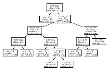
tree.plot_tree(gs.best_estimator_)

[Text(167.4, 199.32, 'X[2] <= 2.45\ngini = 0.667\nsamples = 150\nvalue = [50, 50, 50]'),
 Text(141.64615384615385, 163.07999999999998, 'gini = 0.0\nsamples = 50\nvalue = [50, 0, 0]'),
 Text(193.15384615384616, 163.07999999999998, 'X[3] <= 1.75\ngini = 0.5\nsamples = 100\nvalue = [0, 50, 50]'),
 Text(103.01538461538462, 126.83999999999999, 'X[2] <= 4.95\ngini = 0.168\nsamples = 54\nvalue = [0, 49, 5]'),
 Text(51.50769230769231, 90.6, 'X[3] <= 1.65\ngini = 0.041\nsamples = 48\nvalue = [0, 47, 1]'),
 Text(25.753846153846155, 54.359999999999985, 'gini = 0.0\nsamples = 47\nvalue = [0, 47, 0]'),
 Text(77.26153846153846, 54.359999999999985, 'gini = 0.0\nsamples = 1\nvalue = [0, 0, 1]'),
 Text(154.52307692307693, 90.6, 'X[3] <= 1.55\ngini = 0.444\nsamples = 6\nvalue = [0, 2, 4]'),
 Text(128.76923076923077, 54.359999999999985, 'gini = 0.0\nsamples = 3\nvalue = [0, 0, 3]'),
 Text(180.27692307692308, 54.359999999999985, 'X[2] <= 5.45\ngini = 0.444\nsamples = 3\nvalue = [0, 2, 1]'),
 Text(154.52307692307693, 18.119999999999976, 'gini = 0.0\nsamples = 2\nvalue = [0, 2, 0]'),
 Text(206.03076923076924, 18.119999999999976, 'gini = 0.0\nsamples = 1\nvalue = [0, 0, 1]'),
 Text(283.2923076923077, 126.83999999999999, 'X[2] <= 4.85\ngini = 0.043\nsamples = 46\nvalue = [0, 1, 45]'),
 Text(257.53846153846155, 90.6, 'X[1] <= 3.1\ngini = 0.444\nsamples = 3\nvalue = [0, 1, 2]'),
 Text(231.7846153846154, 54.359999999999985, 'gini = 0.0\nsamples = 2\nvalue = [0, 0, 2]'),
 Text(283.2923076923077, 54.359999999999985, 'gini = 0.0\nsamples = 1\nvalue = [0, 1, 0]'),
 Text(309.04615384615386, 90.6, 'gini = 0.0\nsamples = 43\nvalue = [0, 0, 43]')]

png

python

import graphviz

python

data = tree.export_graphviz(gs.best_estimator_,
                           out_file = None,
                           feature_names = iris.feature_names,
                           class_names = iris.target_names,
                           filled = True,
                           rounded = True,
                           special_characters = True)

python

graph = graphviz.Source(data)

python

graph.render("iris_bonito")

'iris_bonito.pdf'