Regresión lineal
 Jeshua Romero Guadarrama
- 2 Min para leer
- 04 Jul, 2021
Índice de contenido
python
import matplotlib.pyplot as plt
import numpy as np
from sklearn import linear_model
import pandas as pd
Datos de estudio
python
X = np.array([32, 25, 25, 22, 24, 35, 40, 30, 28, 25])
y = np.array([27, 42, 40, 50, 45, 30, 25, 25, 30, 40])
python
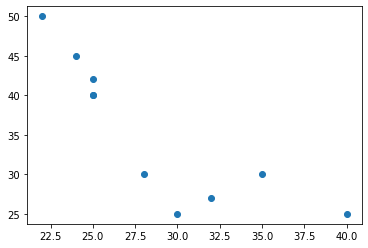
# Nube de puntos
plt.scatter(X, y)
<matplotlib.collections.PathCollection at 0x8f0eaf0>
Mínimos cuadrados “a mano”
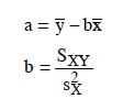
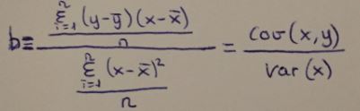
Coeficientes
python
# Coeficiente de regresión (b)
b = sum((y-np.mean(y))*(X-np.mean(X)))/sum((X-np.mean(X))**2)
b
-1.3536754507628292
python
# Ordenada en el origen (a)
a = np.mean(y) - b*np.mean(X)
a
74.11511789181691
Predicciones
python
# Predicciones
# y*=a+b*X
y_pred = a + b * X
y_pred
array([30.79750347, 40.27323162, 40.27323162, 44.33425798, 41.62690707,
       26.73647712, 19.96809986, 33.50485437, 36.21220527, 40.27323162])
python
y
array([27, 42, 40, 50, 45, 30, 25, 25, 30, 40])
Coeficientes de determinación
python
# Sin ajustar
r2 = sum((y_pred - np.mean(y))**2)/sum((y - np.mean(y))**2)
r2
0.7176465181664967
python
n = len(X)
n
10
python
k = 1
python
# Ajustado
r2_adj = 1 - ((n-1)/(n-k-1))*(1-r2)
r2_adj
0.6823523329373088
Mínimos cuadrados con scikit-learn
python
model = linear_model.LinearRegression()
model
LinearRegression()
python
X
array([32, 25, 25, 22, 24, 35, 40, 30, 28, 25])
python
X = X.reshape(-1, 1)
X
array([[32],
       [25],
       [25],
       [22],
       [24],
       [35],
       [40],
       [30],
       [28],
       [25]])
python
y = y.reshape(-1, 1)
y
array([[27],
       [42],
       [40],
       [50],
       [45],
       [30],
       [25],
       [25],
       [30],
       [40]])
python
results = model.fit(X,y)
results
LinearRegression()
Coeficientes
python
# Coeficiente de regresión (b)
results.coef_
array([[-1.35367545]])
python
# Ordenada en el origen (a)
results.intercept_
array([74.11511789])
Predicciones
python
# Predicciones
y_pred_sk = model.predict(X)
y_pred_sk
array([[30.79750347],
       [40.27323162],
       [40.27323162],
       [44.33425798],
       [41.62690707],
       [26.73647712],
       [19.96809986],
       [33.50485437],
       [36.21220527],
       [40.27323162]])
Coeficientes de determinación
python
results.score(X, y)
0.717646518166497
python
results.get_params()
{'copy_X': True, 'fit_intercept': True, 'n_jobs': None, 'normalize': False}
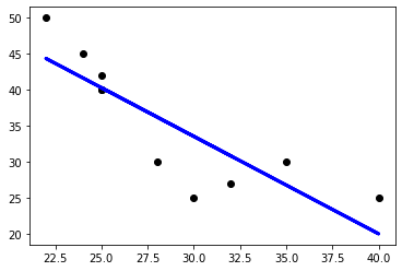
Visualización de predicciones
python
plt.scatter(X, y, color = "black")
plt.plot(X, y_pred, color = "blue", linewidth = 3)
[<matplotlib.lines.Line2D at 0xc7a3a00>]
python
X = X.flatten()
y = y.flatten()
python
y
array([27, 42, 40, 50, 45, 30, 25, 25, 30, 40])
python
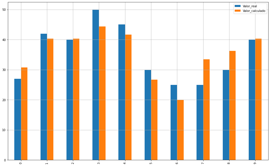
comparison = pd.DataFrame({"Valor_real": y,
                          "Valor_calculado": y_pred})
comparison
| Valor_real | Valor_calculado | |
|---|---|---|
| 0 | 27 | 30.797503 |
| 1 | 42 | 40.273232 |
| 2 | 40 | 40.273232 |
| 3 | 50 | 44.334258 |
| 4 | 45 | 41.626907 |
| 5 | 30 | 26.736477 |
| 6 | 25 | 19.968100 |
| 7 | 25 | 33.504854 |
| 8 | 30 | 36.212205 |
| 9 | 40 | 40.273232 |
python
comparison.plot(kind = "bar", figsize=(16,10))
plt.grid(which="major")
python
residuals = y-y_pred_sk
python
plt.scatter(y_pred_sk, residuals)
<matplotlib.collections.PathCollection at 0xb553820>