
Regresión no lineal
 Jeshua Romero Guadarrama
- 4 Min para leer
- 08 Jul, 2021
Índice de contenido
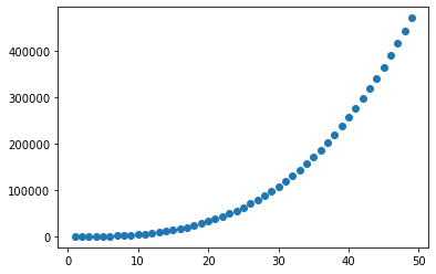
Y = a·X^b
a = 4
b = 3
Y = 4·X^3
python
import matplotlib.pyplot as plt
python
from sklearn import linear_model
Generación de datos
python
a = 4
b = 3
python
X = np.arange(50)
X
array([ 0,  1,  2,  3,  4,  5,  6,  7,  8,  9, 10, 11, 12, 13, 14, 15, 16,
       17, 18, 19, 20, 21, 22, 23, 24, 25, 26, 27, 28, 29, 30, 31, 32, 33,
       34, 35, 36, 37, 38, 39, 40, 41, 42, 43, 44, 45, 46, 47, 48, 49])
python
lista_valores = []
for i in X:
    if i > 0:
        lista_valores.append(i)
python
X = [i for i in X if i>0]
X
[1,
 2,
 3,
 4,
 5,
 6,
 7,
 8,
 9,
 10,
 11,
 12,
 13,
 14,
 15,
 16,
 17,
 18,
 19,
 20,
 21,
 22,
 23,
 24,
 25,
 26,
 27,
 28,
 29,
 30,
 31,
 32,
 33,
 34,
 35,
 36,
 37,
 38,
 39,
 40,
 41,
 42,
 43,
 44,
 45,
 46,
 47,
 48,
 49]
python
X = np.array(X)
X
array([ 1,  2,  3,  4,  5,  6,  7,  8,  9, 10, 11, 12, 13, 14, 15, 16, 17,
       18, 19, 20, 21, 22, 23, 24, 25, 26, 27, 28, 29, 30, 31, 32, 33, 34,
       35, 36, 37, 38, 39, 40, 41, 42, 43, 44, 45, 46, 47, 48, 49])
python
y = a*(X*X*X)
y
array([     4,     32,    108,    256,    500,    864,   1372,   2048,
         2916,   4000,   5324,   6912,   8788,  10976,  13500,  16384,
        19652,  23328,  27436,  32000,  37044,  42592,  48668,  55296,
        62500,  70304,  78732,  87808,  97556, 108000, 119164, 131072,
       143748, 157216, 171500, 186624, 202612, 219488, 237276, 256000,
       275684, 296352, 318028, 340736, 364500, 389344, 415292, 442368,
       470596])
Resolución del problema
python
X
array([ 1,  2,  3,  4,  5,  6,  7,  8,  9, 10, 11, 12, 13, 14, 15, 16, 17,
       18, 19, 20, 21, 22, 23, 24, 25, 26, 27, 28, 29, 30, 31, 32, 33, 34,
       35, 36, 37, 38, 39, 40, 41, 42, 43, 44, 45, 46, 47, 48, 49])
python
y
array([     4,     32,    108,    256,    500,    864,   1372,   2048,
         2916,   4000,   5324,   6912,   8788,  10976,  13500,  16384,
        19652,  23328,  27436,  32000,  37044,  42592,  48668,  55296,
        62500,  70304,  78732,  87808,  97556, 108000, 119164, 131072,
       143748, 157216, 171500, 186624, 202612, 219488, 237276, 256000,
       275684, 296352, 318028, 340736, 364500, 389344, 415292, 442368,
       470596])
python
plt.scatter(X, y)
<matplotlib.collections.PathCollection at 0x39f9d30>
y = a · X^b
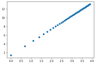
log_y = log_a + b · log_X
python
log_y = np.log(y)
log_y
array([ 1.38629436,  3.4657359 ,  4.68213123,  5.54517744,  6.2146081 ,
        6.76157277,  7.22402481,  7.62461899,  7.97796809,  8.29404964,
        8.57998018,  8.84101431,  9.08114243,  9.30346635,  9.51044496,
        9.70406053,  9.88593439, 10.05740963, 10.2196113 , 10.37349118,
       10.51986167, 10.65942172, 10.79277701, 10.92045585, 11.04292184,
       11.16058398, 11.27380496, 11.38290789, 11.48818185, 11.58988651,
       11.68825597, 11.78350207, 11.87581705, 11.96537593, 12.05233855,
       12.13685118, 12.2190481 , 12.29905284, 12.3769793 , 12.45293272,
       12.52701056, 12.59930322, 12.66989471, 12.73886326, 12.80628183,
       12.87221855, 12.93673717, 12.99989739, 13.06175526])
python
log_X = np.log(X)
log_X
array([0.        , 0.69314718, 1.09861229, 1.38629436, 1.60943791,
       1.79175947, 1.94591015, 2.07944154, 2.19722458, 2.30258509,
       2.39789527, 2.48490665, 2.56494936, 2.63905733, 2.7080502 ,
       2.77258872, 2.83321334, 2.89037176, 2.94443898, 2.99573227,
       3.04452244, 3.09104245, 3.13549422, 3.17805383, 3.21887582,
       3.25809654, 3.29583687, 3.33220451, 3.36729583, 3.40119738,
       3.4339872 , 3.4657359 , 3.49650756, 3.52636052, 3.55534806,
       3.58351894, 3.61091791, 3.63758616, 3.66356165, 3.68887945,
       3.71357207, 3.73766962, 3.76120012, 3.78418963, 3.80666249,
       3.8286414 , 3.8501476 , 3.87120101, 3.8918203 ])
python
plt.scatter(log_X, log_y)
<matplotlib.collections.PathCollection at 0x808fb80>
python
model = linear_model.LinearRegression()
python
X = X.reshape(-1, 1)
python
results = model.fit(log_X.reshape(-1, 1), log_y.reshape(-1, 1))
python
b_calculado = results.coef_
b_calculado
array([[3.]])
python
a_calculada = np.exp(results.intercept_)
a_calculada
array([4.])
python
# y = a · X^b
y = 4 · X ^ 3
Números negativos ó 0
python
X_neg = np.array([-5, -4, 0,  1,  2,  3,  4,  5,  6,  7,  8,  9, 10, 11, 12, 13, 14, 15, 16,
       17, 18, 19, 20, 21, 22, 23, 24, 25, 26, 27, 28, 29, 30, 31, 32, 33,
       34, 35, 36, 37, 38, 39, 40, 41, 42, 43, 44, 45, 46, 47, 48, 49])
X_neg
array([-5, -4,  0,  1,  2,  3,  4,  5,  6,  7,  8,  9, 10, 11, 12, 13, 14,
       15, 16, 17, 18, 19, 20, 21, 22, 23, 24, 25, 26, 27, 28, 29, 30, 31,
       32, 33, 34, 35, 36, 37, 38, 39, 40, 41, 42, 43, 44, 45, 46, 47, 48,
       49])
python
X_neg_log = np.log(X_neg)
X_neg_log
<ipython-input-30-bae9bdb7096a>:1: RuntimeWarning: divide by zero encountered in log
  X_neg_log = np.log(X_neg)
<ipython-input-30-bae9bdb7096a>:1: RuntimeWarning: invalid value encountered in log
  X_neg_log = np.log(X_neg)
array([       nan,        nan,       -inf, 0.        , 0.69314718,
       1.09861229, 1.38629436, 1.60943791, 1.79175947, 1.94591015,
       2.07944154, 2.19722458, 2.30258509, 2.39789527, 2.48490665,
       2.56494936, 2.63905733, 2.7080502 , 2.77258872, 2.83321334,
       2.89037176, 2.94443898, 2.99573227, 3.04452244, 3.09104245,
       3.13549422, 3.17805383, 3.21887582, 3.25809654, 3.29583687,
       3.33220451, 3.36729583, 3.40119738, 3.4339872 , 3.4657359 ,
       3.49650756, 3.52636052, 3.55534806, 3.58351894, 3.61091791,
       3.63758616, 3.66356165, 3.68887945, 3.71357207, 3.73766962,
       3.76120012, 3.78418963, 3.80666249, 3.8286414 , 3.8501476 ,
       3.87120101, 3.8918203 ])
python
# Transformaciones posibles para evitar el problema de los nan y -inf al tomar logaritmos
X = log(1+X-min(X))