
SVM - Práctica de clasificación con SVC (caso sencillo)
 Jeshua Romero Guadarrama
- 2 Min para leer
- 12 Jul, 2021
Índice de contenido
python
import matplotlib.pyplot as plt
from sklearn.svm import SVC
python
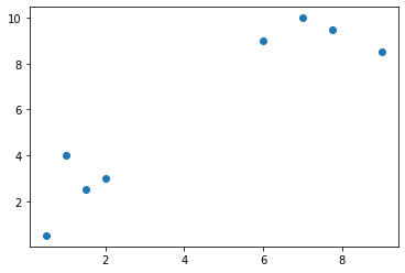
x_coord = [1, 0.5, 2, 1.5, 6, 7, 7.75, 9]
y_coord = [4, 0.5, 3, 2.5, 9, 10, 9.5, 8.5]
y = np.array([0, 0, 0, 0, 1, 1, 1, 1])
python
plt.scatter(x_coord, y_coord)
<matplotlib.collections.PathCollection at 0x9251190>
python
X = np.vstack((x_coord, y_coord)).T
X
array([[ 1.  ,  4.  ],
       [ 0.5 ,  0.5 ],
       [ 2.  ,  3.  ],
       [ 1.5 ,  2.5 ],
       [ 6.  ,  9.  ],
       [ 7.  , 10.  ],
       [ 7.75,  9.5 ],
       [ 9.  ,  8.5 ]])
python
classifier = SVC(kernel='linear')
python
results = classifier.fit(X, y)
python
results.coef_
array([[0.19964497, 0.20023669]])
y_recta = b*x_recta + a
python
results.coef_[0]
array([0.19964497, 0.20023669])
python
b = - results.coef_[0][0]/results.coef_[0][1]
b
-0.9970449172576831
python
a = - results.intercept_[0]/results.coef_[0][1]
a
9.989164696611505
python
x_recta = [i for i in range(13)]
x_recta
[0, 1, 2, 3, 4, 5, 6, 7, 8, 9, 10, 11, 12]
python
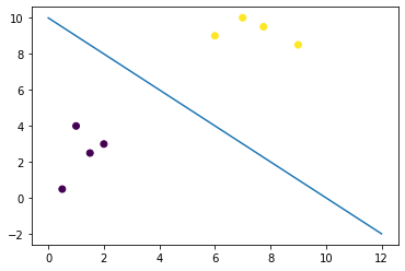
y_recta = b*np.array(x_recta) + a
y_recta
array([ 9.9891647 ,  8.99211978,  7.99507486,  6.99802994,  6.00098503,
        5.00394011,  4.00689519,  3.00985028,  2.01280536,  1.01576044,
        0.01871552, -0.97832939, -1.97537431])
python
plt.plot(x_recta, y_recta)
plt.scatter(x_coord, y_coord, c = y)
<matplotlib.collections.PathCollection at 0xc334100>
python
pt1 = [1.5, 2]
pt2 = [9, 8]
python
X
array([[ 1.  ,  4.  ],
       [ 0.5 ,  0.5 ],
       [ 2.  ,  3.  ],
       [ 1.5 ,  2.5 ],
       [ 6.  ,  9.  ],
       [ 7.  , 10.  ],
       [ 7.75,  9.5 ],
       [ 9.  ,  8.5 ]])
python
nuevos_puntos = np.array([pt1, pt2])
nuevos_puntos
array([[1.5, 2. ],
       [9. , 8. ]])
python
classifier.predict(nuevos_puntos)
array([0, 1])